Algorithmic Design and Techniques

Programming challenges
Algorithmic warm-up
Greedy algorithm
Divide-and-conquer
Dynamic Programming 1
Dynamic Programming 2

Programming challenges

Document: pdf

Algorithmic warm-up

Document: pdf

Fibonacci numbers

Definition: $F_n=\begin{cases} 0 & n=0\\ 1 & n=1\\ F_{n-1}+F_{n-2} & n>1 \end{cases}$

Naive algorithm:

def FibRecurs(n):
    if n <= 1:
        return n
    else:
        return FibRecurs(n-1) + FibRecurs(n-2)

Running time: let $T(n)$ denote the number of lines of code executed by program. So $T(n)=\begin{cases} 2 & n\le 1\\ T(n-1) + T(n-2)+3 & n>1 \end{cases}$ If $n=0,1, T(n)=2>1=F_1>F_0$. If $T(n-1)\ge F_{n-1}$ and $T(n-2)\ge F_{n-2}$, then $T(n)=T(n-1) + T(n-2)+3\ge F_{n-1}+F_{n-2}+3>F_n$ By induction, $T(n)\ge F_n$. This is not acceptable! We keep computing the same $F_n$ again and again, that’s why the algorithm is very slow.

def FibList(n):
    create an array F[0,...,n]
    F[0] <- 0
    F[1] <- 1
    for i from 2 to n:
        F[i] <- F[i-1] + F[i-2]
    return F[n]

$T(n)=2n+2$.

Greatest common divisor (GCD)

Thought: $a=a’+bq$ for some $q$, so $d$ divides $a,b$ iff it divides $a’,b$.

Lemma: gcd(a,b) = gcd(a',b) = gcd(b,a')

def EuclidGCD(a,b):
    if b=0:
        return a
    a' <- the remainder when a is divided by b
    return EuclidGCD(b,a')

For least common multiplier (lcm), a * b = gcd(a,b) * lcm(a,b). Use // for integer divisor, or there would be precision problem when numbers are large.

Big O notation

Definition: $ f(n)=O(g(n))(f $ is Big-O of $ g) $ or $ f \preceq g $ if there exist constants $ N $ and $ c $ so that for all $ n \geq N, f(n) \leq c \cdot g(n) $.

Clarifies growth rate: we care how much runtime scale with input size

Common Rules

Multiplicative constants can be omitted: $7 n^{3}=O\left(n^{3}\right), \frac{n^{2}}{3}=O\left(n^{2}\right)$
$n^{a} \prec n^{b}$ for $0 < a < b$: $n=O\left(n^{2}\right), \sqrt{n}=O(n)$
$n^{a} \prec b^{n}(a>0, b>1)$: $n^{5}=O\left(\sqrt{2}^{n}\right), n^{100}=O\left(1.1^{n}\right)$
$(\log n)^{a} \prec n^{b}(a, b>0)$: $(\log n)^{3}=O(\sqrt{n}), n \log n=O\left(n^{2}\right)$

Smaller terms can be omitted : $n^{2}+n=O\left(n^{2}\right), 2^{n}+n^{9}=O\left(2^{n}\right)$ Consider Fibonacci numbers,

for i from 2 to n: 
    F[i] <- F[i-1] + F[i-2]

This should be $O(n^2)$. Addition between two very large numbers is $O(n)$.

For functions $ f, g: \mathbb{N} \rightarrow \mathbb{R}^{+} $we say that:

$ f(n)=\Omega(g(n)) $ or $ f \succeq g $ if for some $ c $, $ f(n) \geq c \cdot g(n) $ ( $ f $ grows no slower than $ g) $.
$ f(n)=\Theta(g(n)) $ or $ f \asymp g $ if $ f=O(g) $ and $ f=\Omega(g) $ ( $ f $ grows at the same rate as $ g) $.
For functions $ f, g: \mathbb{N} \rightarrow \mathbb{R}^{+} $we say that: $f(n) = o(g(n))$ or $f \prec g$ if $f(n)/g(n) \to 0$ as $n \to \infty (f \text{ grows slower than } g)$.

Pisano period

The modulus of Fibonacci numbers is periodic, the period of mod $m$ is called Pisano period ($P_m$). In order to get $F_n \mod m$, first let n <- n % P_m, then apply naive algorithm.

# Uses python3
def pisano_period(m):
    previous, current = 0, 1
    for i in range(m*m):
        previous, current = current, (previous + current) % m

        if (previous == 0) and (current == 1):
            return i + 1

def get_fibonacci_huge_naive(n, m):
    previous, current = 0, 1

    n = n % pisano_period(m)

    if n <= 1:
        return n
    else:
        for _ in range(n - 1):
            previous, current = current, (previous + current)

    return current % m

Sum of Fibonacci numbers

Property: $S_n = F_0 + F_1 + \dots + F_n = F_{n+2} - 1$ This can be easily proved by induction.

Greedy algorithm

Document: pdf

Definition: Subproblem is a similar problem of smaller size. A greedy choice is called safe choice if there is an optimal solution consistent with this first choice.

In the patient queue problem, safe choice is: the patient with treatment time $t_{\min}$ is the first.

MinTotalWaitingTime(t,n)
waitingTime <- 0
treated <- array of n zeros
for i from 1 to n:
    t_min <- +infty
    minIndex <- 0
    for j from 1 to n:
        if treated[j] == 0 and t[j] < t_min:
            t_min <- t[j]
            minIndex <- j
    waitingTime <- waitingTime + (n-i) * t_min
    treated[minIndex] = 1
return waitingTime

The runtime of MinTotalWaitingTime(t,n) is $O(n^2)$, but this problem can be solved in $O(n\log n)$.

General strategy:

Make a greedy choice
Prove that it is a safe choice
Reduce to a subproblem
Solve the subproblem

Celebration party problem

Divide children into groups, each group with age difference smaller than 2 years, what’s the minimum number of groups?

Let $x_1,\cdots,x_n$ be all children’s ages, think of a group of an interval with length 2. The safe choice is let the left edge start at the minimum $x_j,j\ge 1$, and remove the points included in the interval.

Assume $x_1\le x_2\le\cdots\le x_n$,

def PointsCoverSorted(x1,...,xn):
    segments <- empty list
    left <- 1
    while left <= n:
        (l, r) <- (x_left, x_left+2)
        segments.append((l, r))
        left <- left + 1
        while left <= n and x_left <= r:
            left <- left + 1
    return segments

PointsCoverSorted works in $O(n)$, later sorting is $O(n\log n)$, so Sort + PointsCoverSorted is $O(n\log n)$.

Maximizing Loot

Problem:

Input: Weights $w_1,\cdots,w_n$ and values $v_1,\cdots,v_n$ of $n$ items; capacity $W$.
Output: The maximum total value of fractions of items that fit into a knapsack of capacity $W$.

def BestItem(w1,v1,...wn,vn):
    maxValuePerWeight <- 0
    bestItem <- 0
    for i from 1 to n:
        if w_i > 0:
            if v_1 / w_i > maxValuePerWeight:
                maxValuePerWeight <- v_1 / w_i
                bestItem <- i
    return bestItem

def Knapsack(W,w1,v1,...,wn,vn):
    amounts <- [0,0,...,0]
    totalValue <- 0
    for _ in range(n):
        if W = 0:
            return (totalValue, amounts)
        i <- BestItem(w1,v1,...,wn,vn)
        a <- min(w_i, W)
        totalValue <- totalValue + a * v_i / w_i
        w_i <- w_i - a
        amounts[i] <- amounts[i] + a
        W <- W - a
    return (totalValue, amounts)

The running time of Knapsack is $O(n^2)$. If first sort $v_i/w_i$. Assume $v_1/w_1\ge\cdots\ge v_n/w_n$.

def KnapsackFast(W,w1,v1,...,wn,vn):
    amounts <- [0,0,...,0]
    totalValue <- 0
    for i in range(n):
        if W = 0:
            return (totalValue, amounts)
        # i <- BestItem(w1,v1,...,wn,vn)
        a <- min(w_i, W)
        totalValue <- totalValue + a * v_i / w_i
        w_i <- w_i - a
        amounts[i] <- amounts[i] + a
        W <- W - a
    return (totalValue, amounts)

KnapsackFast itself is $O(n)$, sorting is $O(n\log n)$.

Python implementation:

def get_optimal_value(capacity, weights, values):
    value = 0.
    # write your code here
    n = len(weights)
    items = [(values[i] / weights[i], values[i], weights[i]) for i in range(n)]
    items.sort(key=lambda x: x[0], reverse=True)

    for ratio, v, w in items:
        if capacity == 0:
            break
        a = min(capacity, w)
        value += ratio * a
        capacity -= a

    return value

Collecting Signatures

Problem introduction:

You are responsible for collecting signatures from all tenants of a certain building. For each tenant, you know a period of time when he or she is at home. You would like to collect all signatures by visiting the building as few times as possible. The mathematical model for this problem is the following. You are given a set of segments on a line and your goal is to mark as few points on a line as possible so that each segment contains at least one marked point.

Task: Given a set of $ n $ segments $\left\{\left[a_{0}, b_{0}\right],\left[a_{1}, b_{1}\right], \ldots,\left[a_{n-1}, b_{n-1}\right]\right\}$ with integer coordinates on a line, find the minimum number $ m $ of points such that each segment contains at least one point. That is, find a set of integers $ X $ of the minimum size such that for any segment $ \left[a_{i}, b_{i}\right] $ there is a point $ x \in X $ such that $ a_{i} \leq x \leq b_{i} $.

Procedure:

Sort the end of each segment from small to large: $[a_{\pi(1)}, b_{\pi(1)}], [a_{\pi(2)}, b_{\pi(2)}], \dots, [a_{\pi(n)}, b_{\pi(n)}]$, where $b_{\pi(1)} \leq b_{\pi(2)} \leq \dots \leq b_{\pi(n)}$.
Initialize $X=\varnothing$.
Iterate:
- If $x\in [a_{\pi(k)}, b_{\pi(k)}]$ and $x\in X$, do nothing
- Otherwise, add new $x=b_{\pi(k)}$ into $X$

Python implementation:

Segment = namedtuple('Segment', 'start end')

def optimal_points(segments):
    points = []
    segments.sort(key=lambda s: s.end)
    currentPoint = None
    for s in segments:
        if currentPoint is None or not (s.start <= currentPoint <= s.end):
            currentPoint = s.end
            points.append(currentPoint)

    return points

Maximum Number of Prizes

Problem description

Task. The goal of this problem is to represent a given positive integer $ n $ as a sum of as many pairwise distinct positive integers as possible. That is, to find the maximum $ k $ such that $ n $ can be written as $ a_{1}+a_{2}+\cdots+a_{k} $ where $ a_{1}, \ldots, a_{k} $ are positive integers and $ a_{i} \neq a_{j} $ for all $1 \le i < j \le k$.

Python implementation:

def optimal_summands(n):
    summands = []
    currentPrize = 1

    for i in range(n):
        if 2 * currentPrize + 1 <= n - sum(summands):
            summands.append(currentPrize)
            currentPrize += 1
        else:
            summands.append(n - sum(summands))
            break

    return summands

Test result

Different Summands:
Good job! (Max time used: 4.05/5.00, max memory used: 11403264/536870912.)

Remember that command sum is $O(n)$. Now replace sum with a tracking variable total,

def optimal_summands(n):
    summands = []
    currentPrize = 1
    total = 0

    for i in range(n):
        if 2 * currentPrize + 1 <= n - total:
            summands.append(currentPrize)
            total += currentPrize
            currentPrize += 1
        else:
            summands.append(n - total)
            break

    return summands

Test result

Different Summands:
Good job! (Max time used: 0.05/5.00, max memory used: 11411456/536870912.)

Maximum Salary

Previously, the algorithm in lecture works only in case the input consists of single-digit numbers. For example, for an input consisting of two integers $23$ and $3$ ($23$ is not a single-digit number!) it returns $233$ , while the largest number is in fact $323$ . In other words, using the largest number from the input as the first number is not a safe move.

Your goal in this problem is to tweak the above algorithm so that it works not only for single-digit numbers, but for arbitrary positive integers.

from functools import cmp_to_key

def largest_number(a):
    def _cmp(x, y):
        if x + y < y + x: return -1
        elif x + y > y + x: return 1
        else: return 0
    a = sorted(map(str, a), key=cmp_to_key(_cmp), reverse=True)
    res = ""
    for x in a:
        res += x
    return res

Details for cmp_to_key see Codecademy.

Divide-and-conquer

Document: pdf

Linear search

LinearSearch(A, low, high, key)
    if high < low:
        return NOT_FOUND
    if A[low] = key:
        return low
    return LinearSearch(A, low+1, high, key)

The runtime is $\sum_{i=1}^n c=\Theta(n)$.

Consider a sorted array $A$, from smallest to largest order.

Binary search

$n,n/2,n/4,\cdots, 2, 1,0$, complexity is $\sum_{i=0}^{\log_2 n}c=\Theta(\log_2 n)$. Verify: $2^{\log_2 n}=n.$

Python implementation:

def binary_search(a: list, x: int) -> int:
    left, right = 0, len(a)-1
    # write your code here
    while left <= right:
        mid = (left + right) // 2
        if a[mid] == x:
            return mid
        elif x > a[mid]:
            left = mid + 1
        else:
            right = mid - 1
    return -1

Master theorem

If $T(n)=aT(\lfloor n/b\rfloor)+O(n^d)$, for constraints $a>0,b>1,d\ge 0$, then

If $d>\log_b a, T(n)=O(n^d)$
If $d=\log_b a, T(n)=O(n^d\log n)$
If $d<\log_b a, T(n)=O(n^{\log_b a})$

master

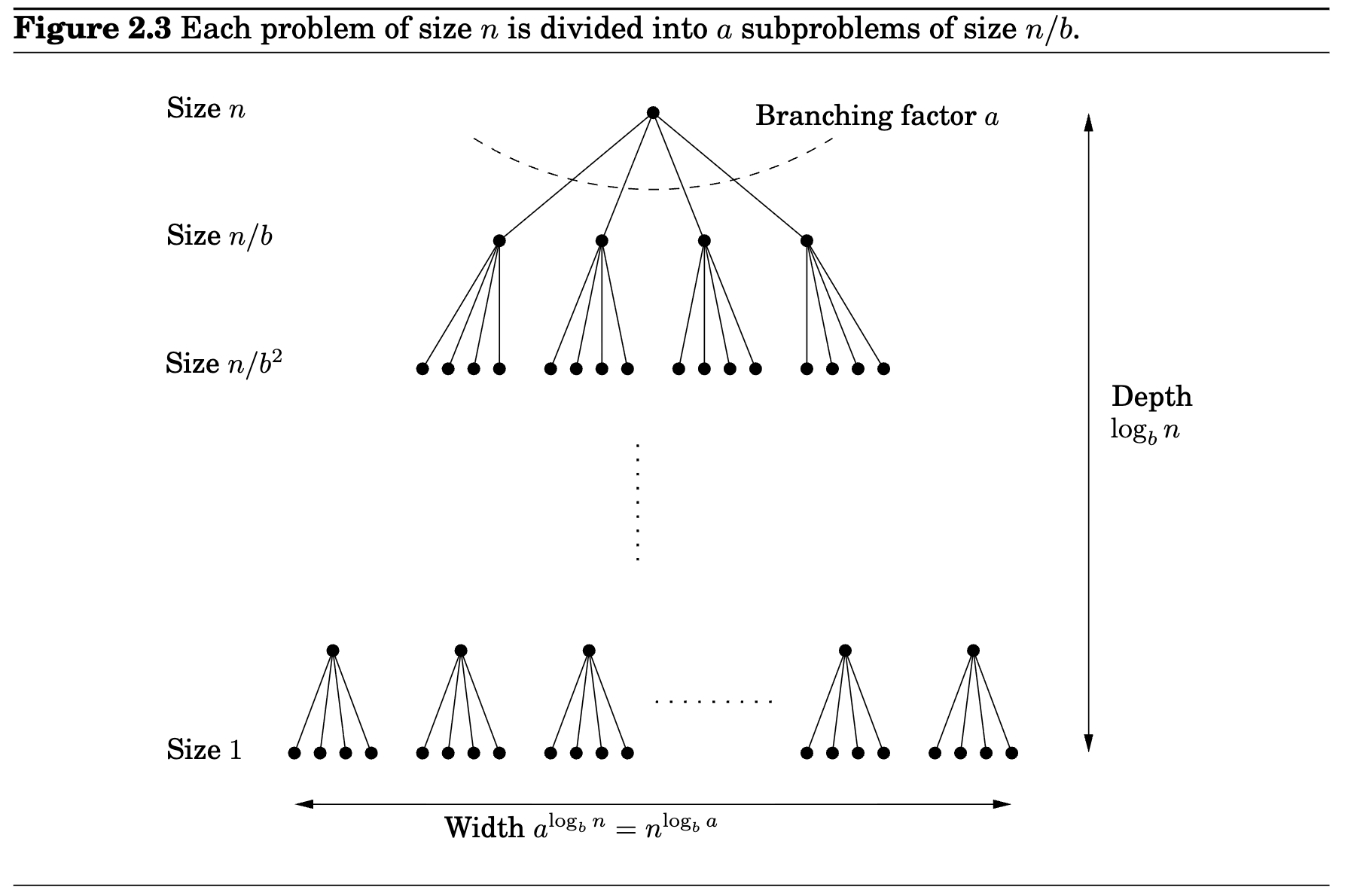
Proof: The amount of work at level $i$ is $a^i O(n/b^i)^d=O(n^d)(a/b^d)^i$. The total work is $\sum_{i=0}^{\log_b n}O(n^d)(a/b^d)^i$.

When $a/b^d<1$ or $d>\log_b a,$ $\sum_{i=0}^{\log_b n}O(n^d)(a/b^d)^i=O(n^d)$
When $a/b^d=1$ or $d=\log_b a,$ $\sum_{i=0}^{\log_b n}O(n^d)(a/b^d)^i=\sum_{i=0}^{\log_b n}O(n^d)=(1+\log_b n)O(n^d)=O(n^d\log n)$
When $a/b^d>1$ or $d<\log_b a,$ $\sum_{i=0}^{\log_b n}O(n^d)(a/b^d)^i=O\bigg(O(n^d)(\frac{a}{b^d})^{\log_b n}\bigg)=\bigg(O(n^d)(\frac{n^{\log_b a}}{n^d})\bigg)=O(n^{\log_b a})$

Majority element

Majority rule is a decision rule that selects the alternative which has a majority, that is, more than half the votes. Given a sequence of elements $ a_{1}, a_{2}, \ldots, a_{n} $, you would like to check whether it contains an element that appears more than $ n / 2 $ times.

def get_majority_element(a, left, right):
    if left == right:
        return -1
    if left + 1 == right:
        return a[left]
    #write your code here
    mid = (left + right) // 2
    m1 = get_majority_element(a, left, mid)
    m2 = get_majority_element(a, mid, right)
    if m1 == m2:
        return m1
    else:
        count1 = sum(1 for i in range(left, right) if a[i] == m1)
        count2 = sum(1 for i in range(left, right) if a[i] == m2)
        if count1 > (right - left) // 2:
            return m1
        elif count2 > (right - left) // 2:
            return m2

    return -1

If enter

5
2 3 9 2 2

The step-by-step picture will be

[0,5): [2,3,9,2,2], mid=2 → result = 2
├── [0,2): [2,3], mid=1 → result = -1
│   ├── [0,1): [2] → 2
│   └── [1,2): [3] → 3
└── [2,5): [9,2,2], mid=3 → result = 2
    ├── [2,3): [9] → 9
    └── [3,5): [2,2], mid=4 → 2
        ├── [3,4): [2] → 2
        └── [4,5): [2] → 2

Selection sort

for i from 1 to n:
    minIndex <- i
    for j from i+1 to n:
        if A[j] < A[minIndex]:
            minIndex <- j
    {A[minIndex] = min A[i,...,n]}
    swap(A[i], A[minIndex])
    {A[1,...,i] is in final position}

Runtime is $O(n^2)$. Pf: $1+2+\cdots+n=n(n+1)/2$.

Other quadratic time sorting algorithms include insertion sort, bubble sort.

Merge sort

def MergeSort(A[1,...,n]):
    if n=1:
        return A
    m <- n//2
    B <- MergeSort(A[1,...,m])
    C <- MergeSort(A[m+1,...,n])
    A' <- Merge(B,C)
    return A'

def Merge(B[1,...,p], C[1,...,q]):
    {B and C are sorted}
    D <- empty array of size p+q
    while B and C are both non-empty:
        b <- the first element of B
        c <- the first element of C
        if b <= c:
            move b from B to the end of D
        else:
            move c from C to the end of D
    move the rest of B or C to the end
    return D

The runtime of MergeSort is $O(n\log n)$. Pf: The runtime of merging is $O(n)$, at most $p+q$ steps are taken to merge B and C. So MergeSort has $T(n)\le 2T(n/2)+O(n)$, then use master theorem.

Exercise: [4-4] Count inversions

Comparison based sorting

Selection sort and merge sort are both comparison based.

Lemma: Any comparison based sorting algo performs $\Omega(n\log n)$ comparisons in the worst case to sort $n$ objects.

Pf: Divide-and-conquer can be considered as a tree with leaves. # of leaves $l$ is at least $n!$, the depth of tree is $d$, then $2^d\ge l\Longrightarrow d\ge \log_2 l$. Thus the runtime is at least $\log_2(n!)\approx \log_2 (\sqrt{2\pi}n^{n+1/2}e^{-n})=\Omega(n\log n)$.

Count sort

Count[1...M] ← [0,...,0]
for i from 1 to n:
    Count[A[i]] ← Count[A[i]] + 1
{k appears Count[k] times in A}
Pos[1...M] ← [0,...,0]
Pos[1] ← 1
for j from 2 to M:
    Pos[j] ← Pos[j−1] + Count[j−1]
{k will occupy range [Pos[k],...,Pos[k+1]-1]}
{or say k starts from index Pos[k]}
for i from 1 to n:
    A′[Pos[A[i]]] ← A[i]
    Pos[A[i]] ← Pos[A[i]] + 1

with complexity $O(n+M)$. Count Sort can only be applied to integer numbers: real numbers cannot play the role of indices of an array.

Quick sort

def Partition(A,l,r):
    x <- A[l]  {pivot}
    j <- l
    for i from l+1 to r:
        if A[i] <= x:
            j <- j + 1
            swap A[j] and A[i]
        {A[l+1,...,j] <= x, A[j+1,...,i] > x}
    swap A[l] and A[j]
    return j

def RandomizedQuickSort(A,l,r):
    if l >= r:
        return
    k <- random number between l and r
    swap A[l] and A[k]
    m <- Partition(A,l,r)
    {A[m] is in the final position}
    RandomizedQuickSort(A,l,m-1)
    RandomizedQuickSort(A,m+1,r)

A nice animation on this.

Efficiency decreases when the split happens unbalancedly. Two cases:

always pick pivot from the edge (use random pivot)
dealing with data that have few unique values (use Partition3)

Design $(m_1,m_2)\leftarrow \text{Partition3}(A,l,r)$, such that

for all $l\le k\le m_1-1,A[k]< x$
for all $m_1\le k\le m_2,A[k]= x$
for all $m_1+1\le k\le r,A[k]> x$

Exercise: [4-3] Partition3.

Dynamic Programming 1

Document: pdf

Money change revisited. This time greedy algo cannot give a safe choice. DP can fix it.

Money change and Primitive calculator are a kind of DP problem.

def optimal_sequence(n):
    v = [float('inf')] * (n + 1)
    v[1] = 0
    for i in range(1, n + 1):
        if i + 1 <= n and v[i + 1] > v[i] + 1:
            v[i + 1] = v[i] + 1
        if i * 2 <= n and v[i * 2] > v[i] + 1:
            v[i * 2] = v[i] + 1
        if i * 3 <= n and v[i * 3] > v[i] + 1:
            v[i * 3] = v[i] + 1

    # backtrack optimal path
    path = [n]
    cur = n
    while cur > 1:
        if cur % 3 == 0 and v[cur // 3] == v[cur] - 1:
            cur //= 3
        elif cur % 2 == 0 and v[cur // 2] == v[cur] - 1:
            cur //= 2
        else:
            cur -= 1
        path.append(cur)
    path.reverse()
    return path

First Bottom-up, then Top-down.

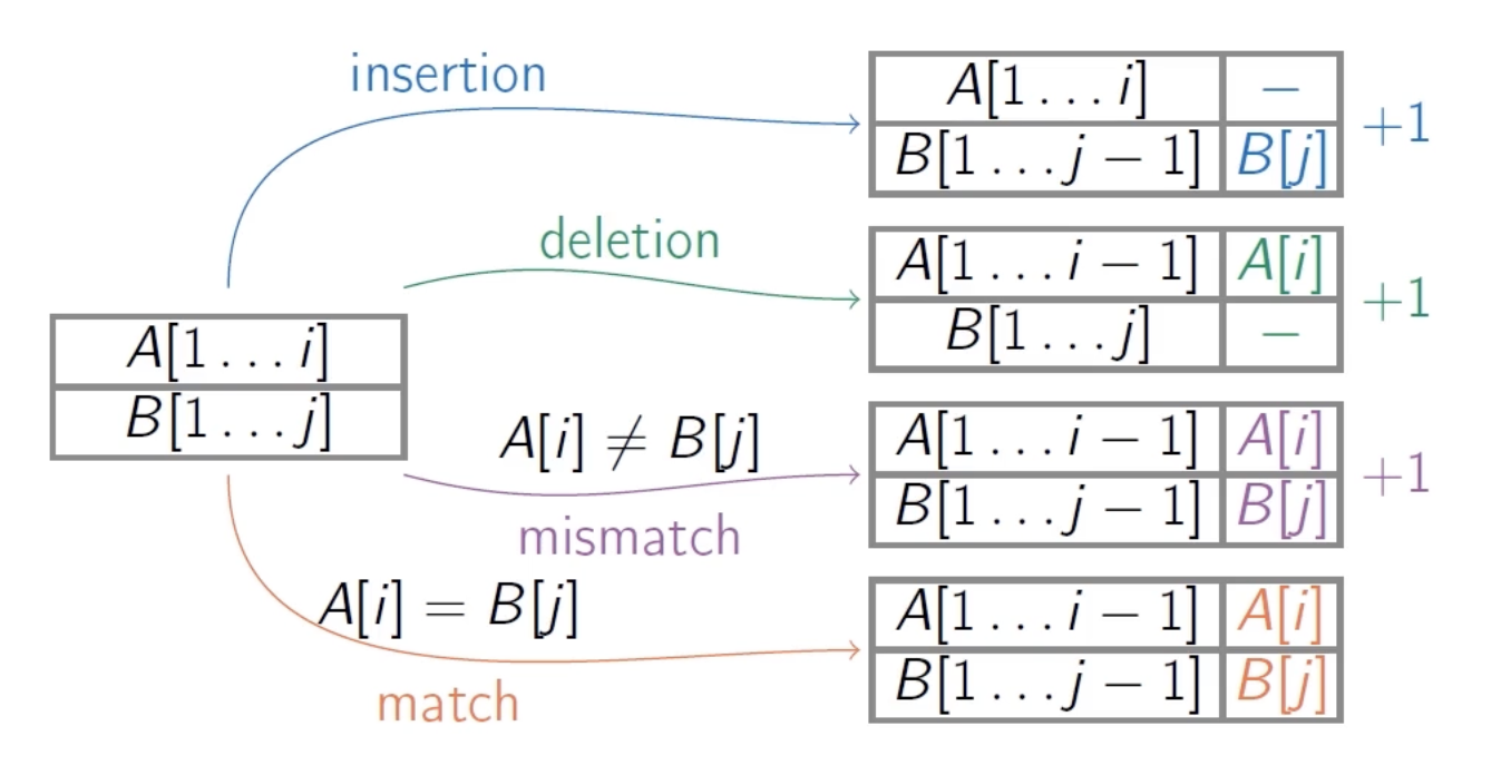
Edit distance is another kind.

edit_distance

Dynamic Programming 2

Document: pdf

Knapsack

knapsack
├── fractional knapsack -> greedy algo
└── discrete knapsack -> greedy does not work!
    ├── with repetitions (unlimited quantities)
    └── without repetitions (one of each item)

Knapsack revisited. Last time we used greedy algo for fractional knapsack. But it doesn’t work for discrete knapsack. Again, DP can fix it. It seems DP is a broader category that can apply to situations when greedy algo is not valid.

Knapsack with repetitions

value(0) <- 0
for w from 1 to W:
    value(w) <- 0
    for i from 1 to n:
        if w_i <= w:
            val <- value(w-w_i) + v_i
            if val > value(w):
                value(w) <- val
return value(W)

Knapsack without repetitions

Subproblems: For $ 0 \leq w \leq W $ and $ 0 \leq i \leq n, \operatorname{value}(w, i) $ is the maximum value achievable using a knapsack of weight $ w $ and items $ 1, \ldots, i $.

The $ i $-th item is either used or not: value $ (w, i) $ is equal to $\max \left\{\text { value }\left(w-w_{i}, i-1\right)+v_{i}, \text { value }(w, i-1)\right\}$

init all value(0, j) <- 0
init all value(w, 0) <- 0
for i from 1 to n:
    for w from 1 to W:
        value(w, i) <- value(w, i-1)
        if w_i <= w:
            val <- value(w-w_i, i-1) + v_i
            if value(w, i) < val:
                value(w, i) <- val
return value(W, n)

Remark

DP question starts from finding the correct subproblem. Then solve subproblem by solving sub-sub-problem. This recurrence relation can be transformed into

iterative algorithm
- solve all subproblems from smaller to bigger ones. (bottom up)
recursive algorithm
- make recursive calls to smaller subsubproblems

Recursive algo can be slow because they compute same thing again and again (e.g. Fibonacci). But here’s a simple technique called memoization: when solving a sub-problem, you store the result in a table.

Usually iterative algorithm is faster.

The running time $O(nW)$ is not polynomial, since $W$ is not the size of input but the value of input. Input size is measured in bits. If $W=10^6$, in binary, $W$ takes $\log_2(10^6)=6$ bits. So the input length includes:

$n$ items: $O(n)$
weights and values, each encoded in $O(\log W)$ bits

In other words, the running time is $O(n 2^{\log W})$.

Placing parentheses

Let $E_{i,j}$ be the subexpression $d_i\ op_i\ \cdots op_{j-1}\ d_j$. Subproblem is, let $M(i,j)$ be the max value of $E_{i,j}$, and $m(i,j)$ be the min value of $E_{i,j}$. $\begin{array}{l}\displaystyle M(i, j)=\max_{i \leq k \leq j-1}\left\{\begin{array}{lll}M(i, k) & o p_{k} & M(k+1, j) \\ M(i, k) & o p_{k} & m(k+1, j) \\ m(i, k) & o p_{k} & M(k+1, j) \\ m(i, k) & o p_{k} & m(k+1, j)\end{array}\right. \quad m(i, j)=\min_{i \leq k \leq j-1}\left\{\begin{array}{lll}M(i, k) & o p_{k} & M(k+1, j) \\ M(i, k) & o p_{k} & m(k+1, j) \\ m(i, k) & o p_{k} & M(k+1, j) \\ m(i, k) & o p_{k} & m(k+1, j)\end{array}\right.\end{array}$

def MinAndMax(i,j):
    min <- +infty
    max <- -infty
    for k from i to j-1:
        a <- M(i,k) op_k M(k+1,j)
        b <- M(i,k) op_k m(k+1,j)
        c <- m(i,k) op_k M(k+1,j)
        d <- m(i,k) op_k m(k+1,j)
        min <- min(min, a, b, c, d)
        max <- max(max, a, b, c, d)
    return (min, max)

def Parentheses(d1, op1, d2, op2, ..., dn):
    for i from 1 to n:
        m(i,i) <- di, M(i,i) <- di
    for s from 1 to n-1:
        for i from 1 to n-s:
            # s=1 -> i=1:(n-1), s=n-1 -> i=1
            j <- i + s
            # keep j-i=s
            min(i,j), M(i,j) <- MinAndMax(i,j)
    return M(1,n)

Algorithmic Design and Techniques

Table of contents

Programming challenges

Algorithmic warm-up

Fibonacci numbers

Greatest common divisor (GCD)

Big O notation

Pisano period

Sum of Fibonacci numbers

Greedy algorithm

Celebration party problem

Maximizing Loot

Collecting Signatures

Maximum Number of Prizes

Maximum Salary

Divide-and-conquer

Linear search

Binary search

Master theorem

Majority element

Selection sort

Merge sort

Comparison based sorting

Quick sort

Dynamic Programming 1

Dynamic Programming 2

Knapsack

Remark

Placing parentheses